KNN (K Nearest Neighbours) Algorithm for Supervised Learning Made Simple

Introduction:

KNN (K Nearest Neighbours) is a classification algorithm which works on a very simple principle. This algorithm is easy to implement on supervised machine learning.
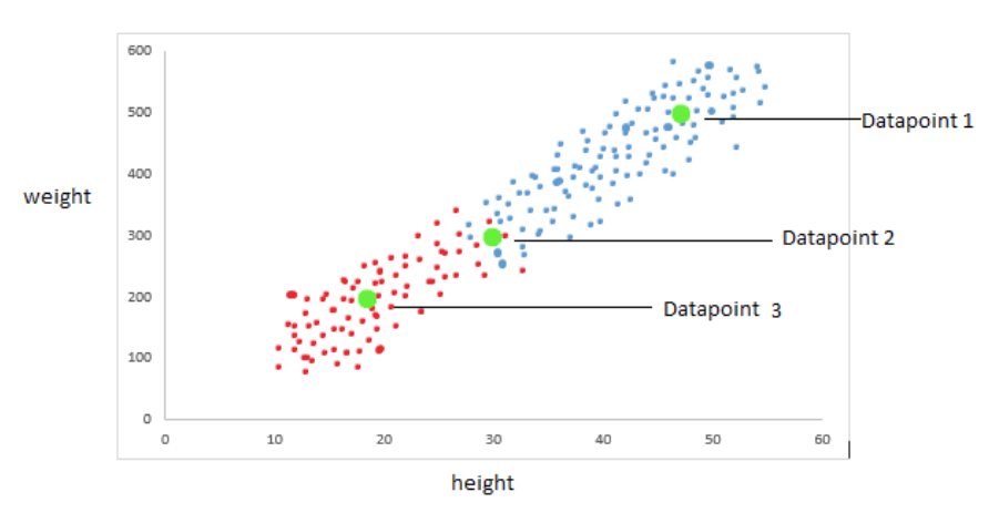
To understand it let’s take some random imaginary dataset of heights and weight of animal 1 and animal 2. The data points are plotted on a scatter plot as shown below.

In the above scatter plot the red points show animal 1 and the blue points show animal 2. There are three additional green dots: data points 1, 2, and 3.

This data is just imaginary so don’t worry about actual weight and height.

The red points indicating animal 1 and blue points indicating animal 2 are the training dataset. If we get any height and weight data points we need to predict if it will be animal 1 or animal 2. Now consider the three green data points; datapoint 1 clearly shows it comes under animal 2 as it is surrounded by blue data points. Similarly, datapoint 3 clearly shows that it comes under the animal 1 category. Datapoint 2 it is surrounded by both the red and green data points so this is where K Nearest Neighbours comes into the picture.

Training Algorithm: The training algorithm simply stores the data.

Prediction Algorithm: The prediction algorithm for test points:

1. Calculates the distance from the given test point to all data points in the data.

2. Sorts the data points in increasing distance from the test point

3. Predicts the majority label of the closest points “K”.
   “K” is the number of closest points.

Understanding K:

Choosing K will affect the category a test point is assigned to:

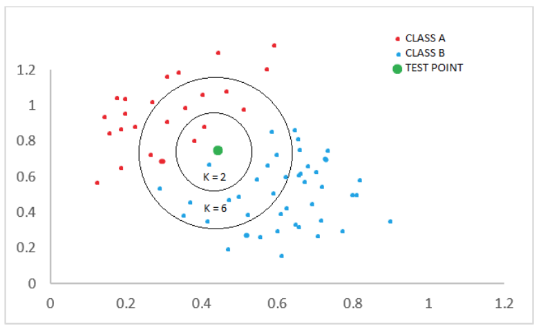
The training points are plotted red points and blue points. There is one green test point.

This is for prediction whether the test point belongs to class A or B.

If we consider K = 2 the test point will come in class A, however if we take K=6 the test point will come under class B as the majority are blue points in K=6.

KNN with Python:

For understanding the KNN algorithm with Python you need to have prior knowledge of sklean, seaborn, and pandas. You need to label the data into features. I have used a dataset called “classified” which contains some values you can try, the same with iris.csv data set.

1
2
3
4
5
6
import pandas as pd
import numpy as np
import matplotlib.pyplot as plt
import seaborn as sns
  %
  matplotlib inline

1
df = pd.read_csv('Classified Data')

1
df.head()

1
2
3
4
5
6
7
8
9
10
11
12
13
14
15
16
17
18
19
20
21
22
23
24
25
26
27
28
29
30
31
32
33
34
35
36
37
38
39
40
41
42
43
44
45
46
47
48
49
50
51
52
53
54
55
56
57
58
59
60
61
62
63
64
65
66
67
68
69
70
71
72
73
74
75
76
77
78
79
80
81
82
83
84
85
86
87
88
89
90
91
92
93
94
95
96
97
98
99
100
101
102
103
104
105
106
107
108
109
<div>
<style scoped>
    .dataframe tbody tr th:only-of-type {
        vertical-align: middle;
    }
    .dataframe tbody tr th {
        vertical-align: top;
    }
    .dataframe thead th {
        text-align: right;
    }
</style>
<table border="1" class="dataframe">
  <thead>
    <tr style="text-align: right;">
      <th></th>
      <th>Unnamed: 0</th>
      <th>WTT</th>
      <th>PTI</th>
      <th>EQW</th>
      <th>SBI</th>
      <th>LQE</th>
      <th>QWG</th>
      <th>FDJ</th>
      <th>PJF</th>
      <th>HQE</th>
      <th>NXJ</th>
      <th>TARGET CLASS</th>
    </tr>
  </thead>
  <tbody>
    <tr>
      <td>0</td>
      <td>0</td>
      <td>0.913917</td>
      <td>1.162073</td>
      <td>0.567946</td>
      <td>0.755464</td>
      <td>0.780862</td>
      <td>0.352608</td>
      <td>0.759697</td>
      <td>0.643798</td>
      <td>0.879422</td>
      <td>1.231409</td>
      <td>1</td>
    </tr>
    <tr>
      <td>1</td>
      <td>1</td>
      <td>0.635632</td>
      <td>1.003722</td>
      <td>0.535342</td>
      <td>0.825645</td>
      <td>0.924109</td>
      <td>0.648450</td>
      <td>0.675334</td>
      <td>1.013546</td>
      <td>0.621552</td>
      <td>1.492702</td>
      <td>0</td>
    </tr>
    <tr>
      <td>2</td>
      <td>2</td>
      <td>0.721360</td>
      <td>1.201493</td>
      <td>0.921990</td>
      <td>0.855595</td>
      <td>1.526629</td>
      <td>0.720781</td>
      <td>1.626351</td>
      <td>1.154483</td>
      <td>0.957877</td>
      <td>1.285597</td>
      <td>0</td>
    </tr>
    <tr>
      <td>3</td>
      <td>3</td>
      <td>1.234204</td>
      <td>1.386726</td>
      <td>0.653046</td>
      <td>0.825624</td>
      <td>1.142504</td>
      <td>0.875128</td>
      <td>1.409708</td>
      <td>1.380003</td>
      <td>1.522692</td>
      <td>1.153093</td>
      <td>1</td>
    </tr>
    <tr>
      <td>4</td>
      <td>4</td>
      <td>1.279491</td>
      <td>0.949750</td>
      <td>0.627280</td>
      <td>0.668976</td>
      <td>1.232537</td>
      <td>0.703727</td>
      <td>1.115596</td>
      <td>0.646691</td>
      <td>1.463812</td>
      <td>1.419167</td>
      <td>1</td>
    </tr>
  </tbody>
</table>
</div>

1
2
from sklearn.preprocessing
import StandardScaler

1
2
scaler = StandardScaler()
scaler.fit(df.drop('TARGET CLASS', axis = 1))

StandardScaler(copy=True, with_mean=True, with_std=True)

1
scaled_features = scaler.transform(df.drop('TARGET CLASS', axis = 1))

1
feature = pd.DataFrame(scaled_features, columns = df.columns[: -1])

1
2
from sklearn.model_selection
import train_test_split

1
X_train, X_test, y_train, y_test = train_test_split(scaled_features, df['TARGET CLASS'], test_size = 0.30)

1
2
from sklearn.neighbors
import KNeighborsClassifier

1
knn = KNeighborsClassifier(n_neighbors = 1)

1
knn.fit(X_train, y_train)

KNeighborsClassifier(algorithm=‘auto’, leaf_size=30, metric=‘minkowski’, metric_params=None, n_jobs=None, n_neighbors=1, p=2, weights=‘uniform’)

1
pred = knn.predict(X_test)

1
2
from sklearn.metrics
import classification_report, confusion_matrix

1
print(confusion_matrix(y_test, pred))

1
print(classification_report(y_test, pred))

1

Try this with different values of n_neighbors and check for accuracy. Also try to change the train and test split ratio.